The fastest way to cut your LLM bill in half is to stop routing every query through your most expensive model. Most enterprise AI pipelines use a single frontier model for everything — classification, extraction, summarization, generation — despite the fact that 60–80% of those tasks could be handled by a model costing 10–100× less.
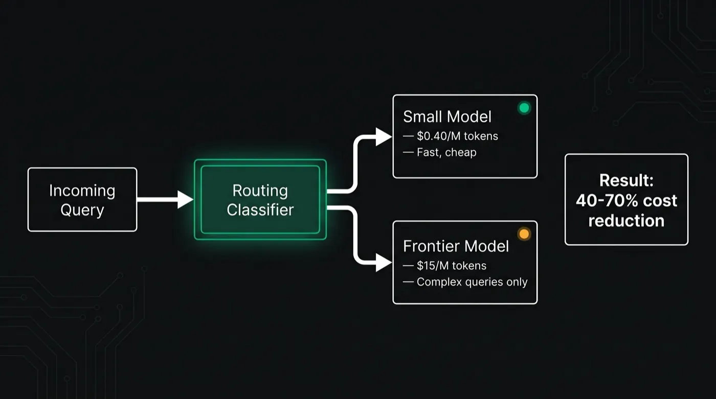
LLM model routing is the technique that fixes this. A lightweight router inspects each incoming query, estimates its complexity, and sends it to the cheapest model capable of answering correctly. Complex or high-stakes queries go to frontier models. Routine tasks go to smaller, cheaper alternatives. Quality stays constant. Costs drop immediately. Routing is one of the five high-leverage techniques covered in our guide to LLM cost optimization.
Loupe by LeanLM (not affiliated with Google’s LearnLM educational AI) measures what AI workloads cost in energy per request — this post covers LLM model routing for cost reduction.
Key Takeaways
- What it is: LLM model routing automatically sends each query to the cheapest model that can answer it correctly, instead of paying frontier prices for every request.
- What it saves: most enterprise teams see 40–70% cost reduction in production; published research (RouteLLM, FrugalGPT) reaches 2× to 98% on specific benchmarks at equal quality.
- How it's done: three architectures — confidence-based cascading, pre-inference classification, and embedding-based routing — optionally combined with policy rules that route by customer tier, budget, or SLA.
- How to start: deploy a two-model confidence cascade on your most predictable query types; no training data required, and it captures savings immediately.
Research from Stanford puts the waste at 50–90% of total inference spend (Chen et al., FrugalGPT, 2023). Model routing is the most direct way to capture it.
Definition
LLM model routing is the practice of automatically directing each query to the cheapest model capable of answering it correctly. A router classifies each request by difficulty or task type — before or during inference — and maps it to the optimal model from a portfolio. The goal is to pay only for the intelligence each task actually requires.
Why Routing Works: The Capability Gap Is Real
Frontier models are overqualified for most production tasks. Not every query needs the reasoning depth of GPT-5.5 or Claude Opus 4.8 — and for tasks where a smaller model performs identically, using a frontier model is pure waste.
Consider what a typical enterprise AI pipeline actually processes:
- Intent classification — what category does this request fall into? (binary or N-way)
- Entity extraction — pull names, dates, amounts from unstructured text
- Template-based summarization — condense a document into a fixed structure
- Structured JSON generation — convert natural language into a schema
- FAQ and policy lookup responses — answer from a fixed knowledge base
- Complex reasoning and generation — nuanced responses, multi-step problems
The first five tasks are commodity inference. A 7B or 13B model adapted via LoRA fine-tuning handles them at equal quality on most workloads. Only the last — complex reasoning and free-form generation where quality variance matters — benefits from frontier intelligence. Routing identifies which category each query falls into and prices accordingly.
Three Routing Architectures
There are three proven approaches to LLM routing. Each makes different tradeoffs between implementation complexity, latency, and accuracy.
Confidence-Based Cascading
Try the cheapest model first. If its response confidence is above a threshold, return it. If not, escalate to a more capable model. Repeat up the capability ladder until confidence is met or the frontier model responds.
Advantages: simple to implement, no training data required, naturally handles edge cases. Disadvantages: low-confidence queries incur latency from multiple model calls before escalating.
FrugalGPT (Chen et al., Stanford, 2023) implements a three-model cascade and achieves up to 98% cost reduction on HellaSwag, MMLU, and CommonsenseQA vs. GPT-4 alone. arxiv:2305.05176 ↗
For coding tasks specifically, the harder question is which fallback model to escalate to once retries run out: our 36-model bake-off found the top scorers all reason before answering. We measured Qwen 3.8 27B on one R9700 as one candidate for that escalation tier.
Pre-Inference Classification
Train a lightweight classifier on samples of your production queries, labeled with which model produced acceptable quality. At inference time, classify first — before any LLM call — and route directly to the predicted best model. No wasted inference on queries you'll escalate anyway.
Advantages: single LLM call per query, no latency penalty. Disadvantages: requires labeled training data from your specific workload; classifier accuracy caps at training data quality.
RouteLLM (Ong et al., 2024) trains a matrix factorization and Bradley-Terry classifier on human preference data, achieving 2× cost savings while maintaining 95% of GPT-4 quality. arxiv:2406.18665 ↗
Embedding-Based Routing
Embed each query and compare it against a library of historical queries with known optimal model assignments. Route to the model that worked best for semantically similar past queries. Improves automatically as you accumulate production data.
Advantages: improves over time, captures subtle task-specific patterns, no manual labeling needed beyond initial setup. Disadvantages: higher latency from embedding computation; cold-start problem with new query types.
Demonstrated effective in production deployments where query types are diverse and overlap with historical patterns. Works best when combined with a fallback cascade for novel query types.
| Approach | Training data | Latency | Setup effort | Best for |
|---|---|---|---|---|
| Cascade | None | Higher (multi-call) | Low | Fast start, unknown query mix |
| Classifier | Required (labeled) | Lowest (single call) | Medium | High volume, stable query types |
| Embedding | Minimal (accumulates) | Medium | Medium | Diverse queries, improving over time |
Most production systems combine approaches — e.g. a classifier for known query types with a cascade fallback for novel ones.
What Routing Can and Cannot Replace
Routing is not a universal solution. It works best when your query distribution is predictable and you have sufficient volume on each task type to measure quality empirically. Understanding its limits prevents misconfigured deployments.
Tasks where routing typically captures full savings:
- Classification with 3–20 predefined categories
- Structured data extraction from predictable document formats
- Summarization of short, well-structured documents
- JSON generation with a fixed schema
- Sentiment analysis and intent detection
- Lookup-style responses from a fixed knowledge base
Tasks where frontier quality is harder to replace:
- Multi-step reasoning across ambiguous or contradictory inputs
- Novel creative generation where quality judgments are subjective
- High-stakes decisions with significant downside risk (medical, legal)
- Long-form synthesis across many documents with nuanced judgment
The key question is not "is routing safe?" but "for which specific tasks on my actual workload does a smaller model match frontier quality?" This requires running evals on your data, not assuming benchmark performance translates. See when a small model is good enough for a measured example: pass rate and energy per task on the same coding tasks, small model vs large.
Policy-Based and Tier-Based Routing
Everything above routes on a single axis: query difficulty. But difficulty is not the only thing worth routing on. In real products — especially SaaS with multiple pricing tiers — the more valuable routing dimension is often who is asking, not just what they asked. This is policy-based routing: a rules layer that sits on top of (or instead of) difficulty-based routing and decides the model ceiling per request from business context.
The most common pattern is tier-based routing. You map each customer tier to a model or a model ceiling — free-tier traffic to a small open model, paid tiers to a mid-size model, enterprise accounts to a frontier model or a full difficulty cascade. The economics are straightforward: a free user generating zero revenue should not be answered by your most expensive model, while a six-figure enterprise account usually should get frontier quality regardless of how trivial any single query looks. Routing by tier protects margin on low-revenue traffic and reserves frontier spend for the accounts that pay for it.
Tier is just one policy input. Production routers in 2026 increasingly combine several: a per-customer or per-tier cost budget that caps spend over a billing window, a latency or SLA target that forces a faster model for time-sensitive endpoints, and compliance or data-residency rules that pin certain workloads to specific providers. The router evaluates these policy constraints first, then applies difficulty-based routing within whatever envelope the policy allows. Policy decides the ceiling; difficulty decides where under that ceiling each query lands.
Rule-Based vs. Learned Routers: Signal, Latency, and Verification
The three architectures above are all learned routers — they infer difficulty from data. In production most stacks also contain a fourth kind that predates them: the hand-written rule. Comparing all four on the dimensions that actually govern a deployment — what signal the router reads, what latency it adds, and how you verify it is deciding correctly — is more useful than comparing them on savings claims.
| Router type | Routing signal | Added latency | How you verify it | Where it wins |
|---|---|---|---|---|
| Rule-based | Hand-written conditions on endpoint, prompt template, customer tier, or payload size | Effectively none — a branch in your own code | Rule-coverage audit: what share of traffic falls through to the default branch | Small, stable query sets; policy and compliance ceilings |
| Confidence cascade | The cheap model's own confidence — logprobs, or a verifier model's score | One extra model call, but only on escalation | Escalation rate plus sampled quality on the share that was not escalated | No labeled data; unknown or shifting query mix |
| Trained classifier | Predicted difficulty from labeled samples of your own traffic | One small-model forward pass before the LLM call | Held-out routing accuracy against the labels, tracked for drift | High volume with stable, well-understood query types |
| Embedding similarity | Nearest historical queries with known best-model outcomes | An embedding call plus a vector lookup | Neighbor-agreement rate, and cold-start miss rate on novel queries | Diverse queries that overlap with accumulated history |
Latency is expressed as work added per request rather than fixed milliseconds, because the absolute figure depends entirely on your classifier size, embedding model, and network path — measure it on your own stack rather than trusting a published number. The signal column is the useful discriminator: rule-based routers read metadata you already have, learned routers read the query itself.
The practical consequence is that rule-based and learned routers are complements, not alternatives. Rules encode the constraints you can state in advance — this endpoint must stay on a compliant provider, this tier never gets the frontier model — and a learned router picks the cheapest capable model inside whatever envelope the rules leave open. Teams that skip the rules layer end up encoding business policy as training labels, which is both harder to audit and harder to change.
When Routing Actually Saves Money: The Break-Even Formula
For a two-model cascade, the expected cost per query is the cheap model's cost plus the escalation rate times the frontier model's cost. It helps to know what one request actually costs on each side of the cascade before running this math:
cost per query = Ccheap + (e × Cfrontier), where e is the fraction of queries that escalate.
Setting that below the cost of always calling the frontier model gives the break-even condition: e < 1 − (Ccheap ÷ Cfrontier). The headline result is how forgiving this is. If the cheap model costs one twentieth of the frontier model, the cascade wins at any escalation rate below 95% — which is why cascades are nearly always worth trying even before you know your query mix. The cost risk of a badly calibrated cascade is small; the quality risk of a permissive threshold is what deserves the attention.
A pre-inference classifier has no wasted call, so its expected cost is simply the volume-weighted blend — pcheap × Ccheap + (1 − pcheap) × Cfrontier — which is always at or below the frontier cost. Its exposure is not cost but misroutes: every query the classifier sends down that the frontier model should have handled is a silent quality regression, with no confidence signal to catch it. That asymmetry is the real reason to start with a cascade and graduate to a classifier only once you have labels.
If latency rather than cost is your binding constraint, invert the same logic: a cascade adds a full extra model call on the escalated share, so it degrades tail latency exactly where quality matters most, while a classifier adds a small fixed cost to every request and leaves the tail alone.
How to Choose a Routing Approach and Evaluate Routing Tools
Start with the approach, then pick the tooling. The decision between the three architectures comes down to two questions: do you have labeled data from your own workload, and how predictable is your query mix?
- No labeled data, mixed or unknown queries → start with a cascade. It needs no training data and captures savings on day one.
- High volume, stable and well-understood query types → invest in a classifier. The single-call latency win compounds at scale once you have labeled samples.
- Diverse queries that overlap with history and grow over time → use embedding-based routing, ideally with a cascade fallback for cold-start query types.
When you evaluate a routing platform — build vs. buy — judge it on four capabilities rather than the headline savings number:
- Policy support — can it route on customer tier, budget, and SLA, or only on query difficulty? Single-axis routers leave the largest margin lever on the table.
- Eval tooling — does it measure quality on your query distribution, not benchmark averages? Routing calibrated on the wrong distribution silently degrades output.
- Observability — does it expose escalation rate, per-tier cost, and quality drift so you can catch a misconfigured threshold before users do? Pairing routing with dedicated LLM cost tracking tools closes this loop.
- Model-portfolio breadth — how many providers and model sizes can it route across? A wider portfolio means more places to land a query at the right price.
There is no single "best" tool — the right choice is the one whose policy model and eval tooling match how your traffic actually behaves. That is the question worth answering before you write any routing code.
Production Case Studies
Research Foundations
How to Build Your First Router
The fastest path to production routing starts with the cascade approach — no training data required, and it immediately captures savings on your most predictable query types.
- Pick your two-model pair — a cheap model for commodity tasks (e.g., gpt-5.4-nano, Claude Haiku 4.5, or a small open model like Qwen3) and your current frontier model as fallback
- Define your quality signal — how do you know a response is "good enough"? Options: logprob confidence, a lightweight verifier model, human review on a sample, or a downstream metric (e.g., downstream click rate, user satisfaction)
- Set your confidence threshold — run the cheap model on 100–500 representative queries, score outputs, and find the threshold where quality matches your frontier model
- Deploy the cascade — call cheap model first; if confidence exceeds threshold, return; otherwise call frontier model
- Monitor and calibrate — track escalation rate (% of queries hitting frontier model), quality signal distribution, and cost per query over time; the LLM cost tracking tools compared here automate this measurement
A well-calibrated cascade typically escalates 15–35% of queries to the frontier model, with the remainder handled by the cheaper alternative. Starting escalation rate above 50% usually indicates the threshold is too conservative; below 5% often means the threshold is too permissive. For compounding savings, apply prompt compression to the inputs before either model in the cascade processes them.
"The hardest part of model routing is not the engineering — it's defining what 'good enough' means for each task type on your specific production data. Once you have that, the routing logic is straightforward."
Frequently Asked Questions
What is LLM model routing?
LLM model routing automatically directs each incoming query to the cheapest model capable of answering it correctly. Instead of using one frontier model for everything, a lightweight router classifies the difficulty of each query and sends simple requests to smaller, cheaper models while escalating complex ones to frontier models.
How much cost can LLM model routing save?
Research from RouteLLM (Ong et al., 2024) shows 2× cost reduction while maintaining 95% of GPT-4 quality. FrugalGPT (Chen et al., 2023) demonstrates up to 98% cost reduction with equal or better accuracy on specific benchmarks. In production, most enterprise teams see 40–70% savings after implementing routing.
Does model routing reduce quality?
When calibrated correctly, model routing does not reduce output quality on your specific workload. The key is evaluating on your own query distribution, not benchmark averages. Tasks where smaller models match frontier quality include: classification, entity extraction, structured JSON generation, summarization of short documents, and FAQ responses.
What types of LLM routing exist?
Three main approaches: (1) Cascade routing — try a cheap model first, escalate to a more expensive model if confidence is low; (2) Classifier routing — train a lightweight classifier to predict which model each query needs before any inference; (3) Embedding-based routing — use semantic similarity to match queries to model strengths based on historical performance data.
How do you build an LLM router?
The simplest router is a confidence-threshold cascade: call a cheap model, check confidence from logprobs or a verifier, and escalate to a frontier model if confidence is below your threshold. More sophisticated routers train a binary classifier on labeled samples of your production queries — this gets more accurate but requires representative training data.
What is the difference between LLM routing and model cascading?
Cascading tries cheap models first and escalates based on confidence — it always starts with the cheapest option. Routing classifies difficulty before any inference and sends the query directly to the right model — no wasted calls. Cascading is easier to implement; routing is more efficient for predictable query types.
What signals do LLM routers use to classify query complexity?
It depends on the router type. Rule-based routers read metadata you already have — which endpoint was called, which prompt template is in use, the customer's tier, or the size of the payload. Learned routers read the query itself: a confidence cascade uses the cheap model's own output signal (token logprobs, or a separate verifier model's score), a trained classifier uses features learned from labeled samples of your production traffic, and an embedding router uses semantic similarity to historical queries with known best-model outcomes. Surface heuristics such as raw character length or vocabulary rarity are weak proxies on their own — they correlate with difficulty but misclassify short hard questions and long easy ones.
How much latency does an LLM router add?
It varies by architecture, and you should measure it on your own stack rather than trust a published figure. A rule-based router adds effectively nothing — it is a branch in your own code. A trained classifier adds one small-model forward pass before the LLM call. An embedding router adds an embedding call plus a vector lookup. A confidence cascade is the outlier: it adds no latency on the queries it handles directly, but a fully duplicated model call on the ones it escalates, so it degrades tail latency rather than average latency. If your constraint is p95 or p99 rather than mean response time, prefer a classifier over a cascade.
How do you verify that an LLM router is making accurate decisions?
Verification differs by architecture, and each has a distinct failure mode to watch. For a cascade, track escalation rate together with sampled quality on the share that was not escalated — that non-escalated share is where silent regressions hide. For a trained classifier, measure held-out routing accuracy against your labels and re-check it on a schedule, because query distributions drift while the classifier does not. For an embedding router, watch neighbor-agreement rate and the cold-start miss rate on query types absent from history. For rule-based routing, audit what share of traffic falls through to the default branch. Across all four, the meaningful metric is end-task quality on your own production distribution — routing accuracy against a benchmark tells you very little about your workload.
How do I calculate whether model routing will save money?
For a two-model cascade, expected cost per query is Ccheap + (e × Cfrontier), where e is the escalation rate. That beats always calling the frontier model whenever e < 1 − (Ccheap ÷ Cfrontier). Because the price spread between tiers is wide, this condition is easy to satisfy: a cheap model costing one twentieth of the frontier model makes the cascade cheaper at any escalation rate below 95%. For a pre-inference classifier there is no wasted call, so expected cost is the volume-weighted blend pcheap × Ccheap + (1 − pcheap) × Cfrontier, which is always at or below frontier cost. In both cases the binding constraint is quality, not arithmetic.
What is the difference between a rule-based router and a learned router?
A rule-based router applies hand-written conditions to metadata you already have — endpoint, prompt template, customer tier — and adds no latency, but it can only encode what you can state in advance. A learned router infers difficulty from the query itself, via confidence, a trained classifier, or embedding similarity, and adapts to patterns you did not anticipate at the cost of added latency and an evaluation burden. They are complements rather than alternatives: rules express business and compliance constraints as a ceiling, and the learned router picks the cheapest capable model within whatever envelope the rules leave open. Encoding business policy as training labels instead of rules makes it harder to audit and harder to change.
What's the best tool for routing AI queries to the cheapest model?
There is no single best routing tool — the right choice depends on your needs. Evaluate routing platforms on four things: policy support (can it route by query difficulty AND by customer tier, budget, or SLA?), eval tooling (can it measure quality on your own query distribution, not just benchmarks?), observability (per-tier cost, escalation rate, and quality tracking), and model-portfolio breadth (how many providers and model sizes it can route across). As of 2026, open frameworks like RouteLLM cover difficulty-based routing well, while production teams often add policy logic on top. Loupe measures what each routing configuration costs in energy per request on a stated hardware boundary, before you commit to a tool.
How do I route different customer tiers to different models?
Tier-based routing is a policy layer on top of (or instead of) difficulty-based routing. In your router configuration, map each customer tier to a model or model ceiling — for example, free-tier traffic to a small open model, paid tiers to mid-size models, and enterprise tiers to frontier models or a difficulty-based cascade. Attach a per-tier cost budget and latency/SLA target so the router enforces the right ceiling per request. This lets you protect margins on low-revenue traffic while reserving frontier quality for the accounts that pay for it.